Modeling Broadband Access

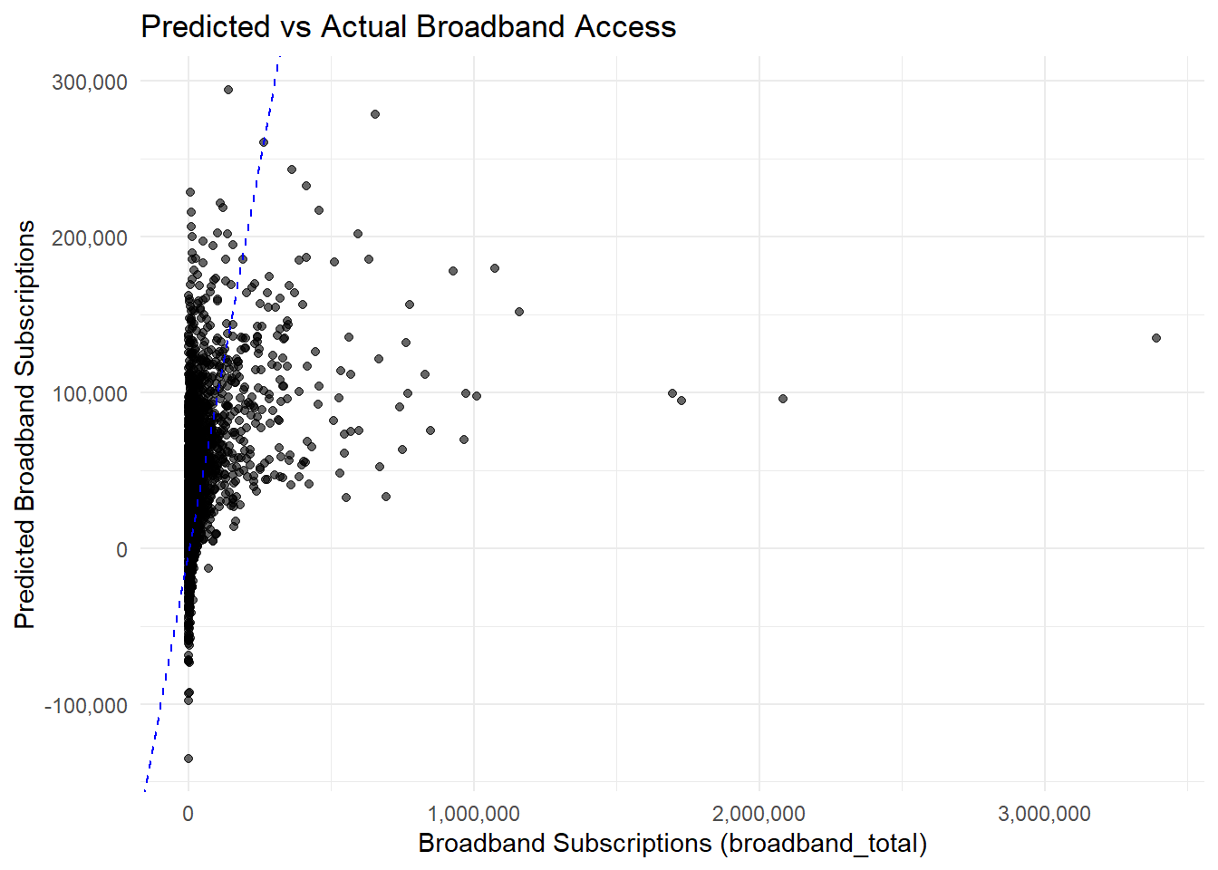
To better understand the factors influencing broadband access across U.S. counties, we developed a linear regression model. The outcome variable is the percentage of households with broadband internet subscriptions. The model includes five key predictors:

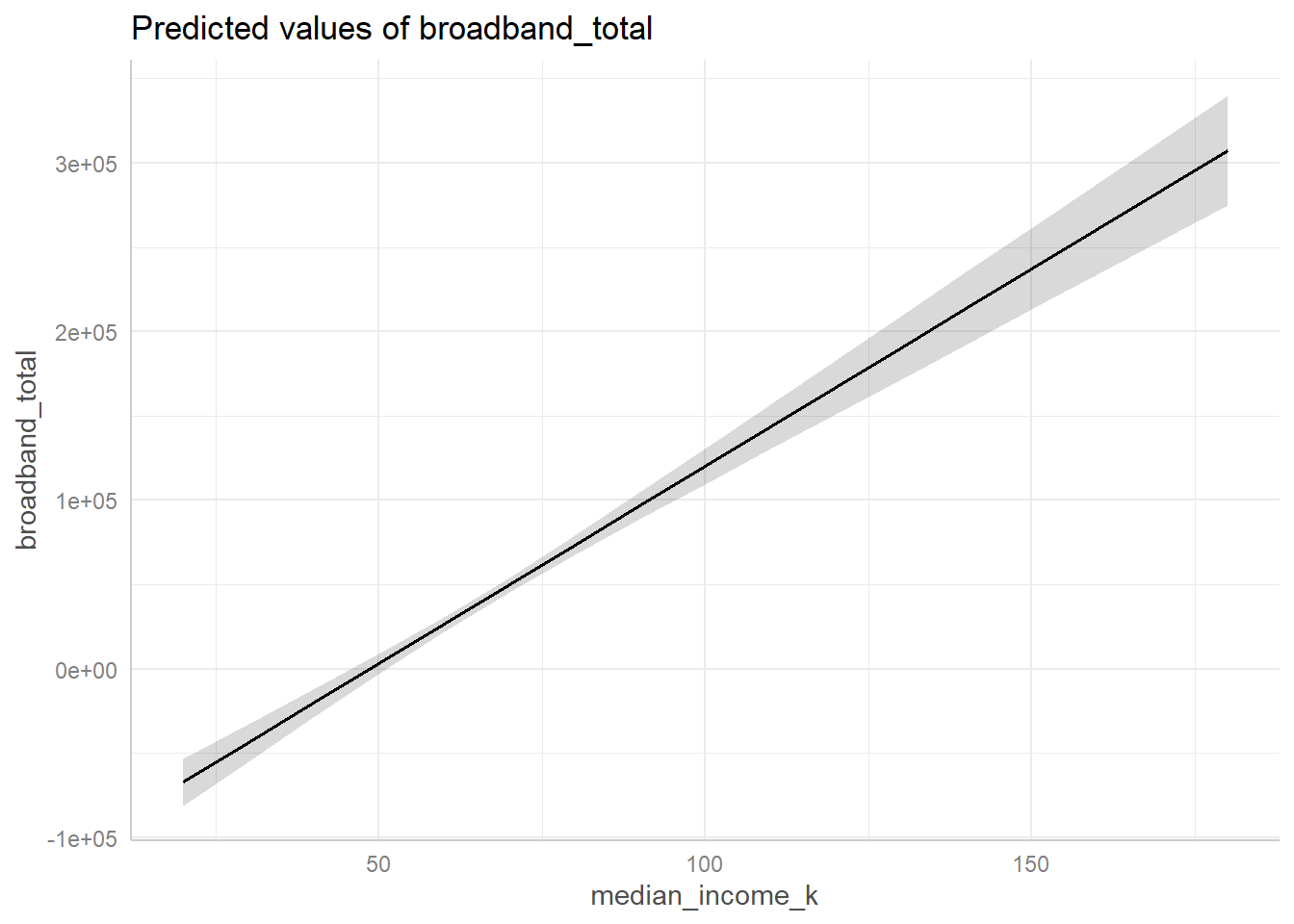
Median household income (in thousands of dollars),
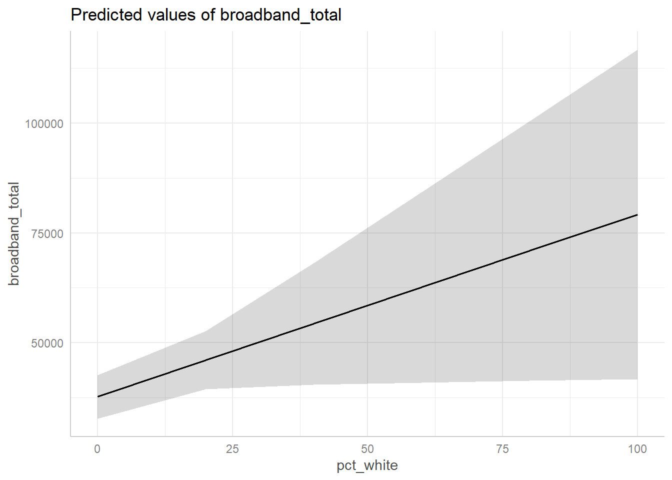
Percentage of the population identifying as White,
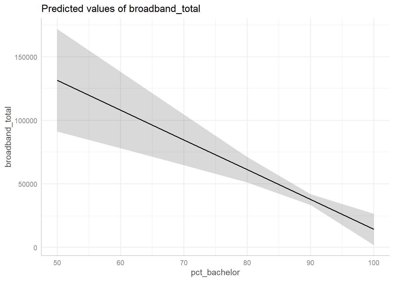
Percentage of adults with a bachelor’s degree, and
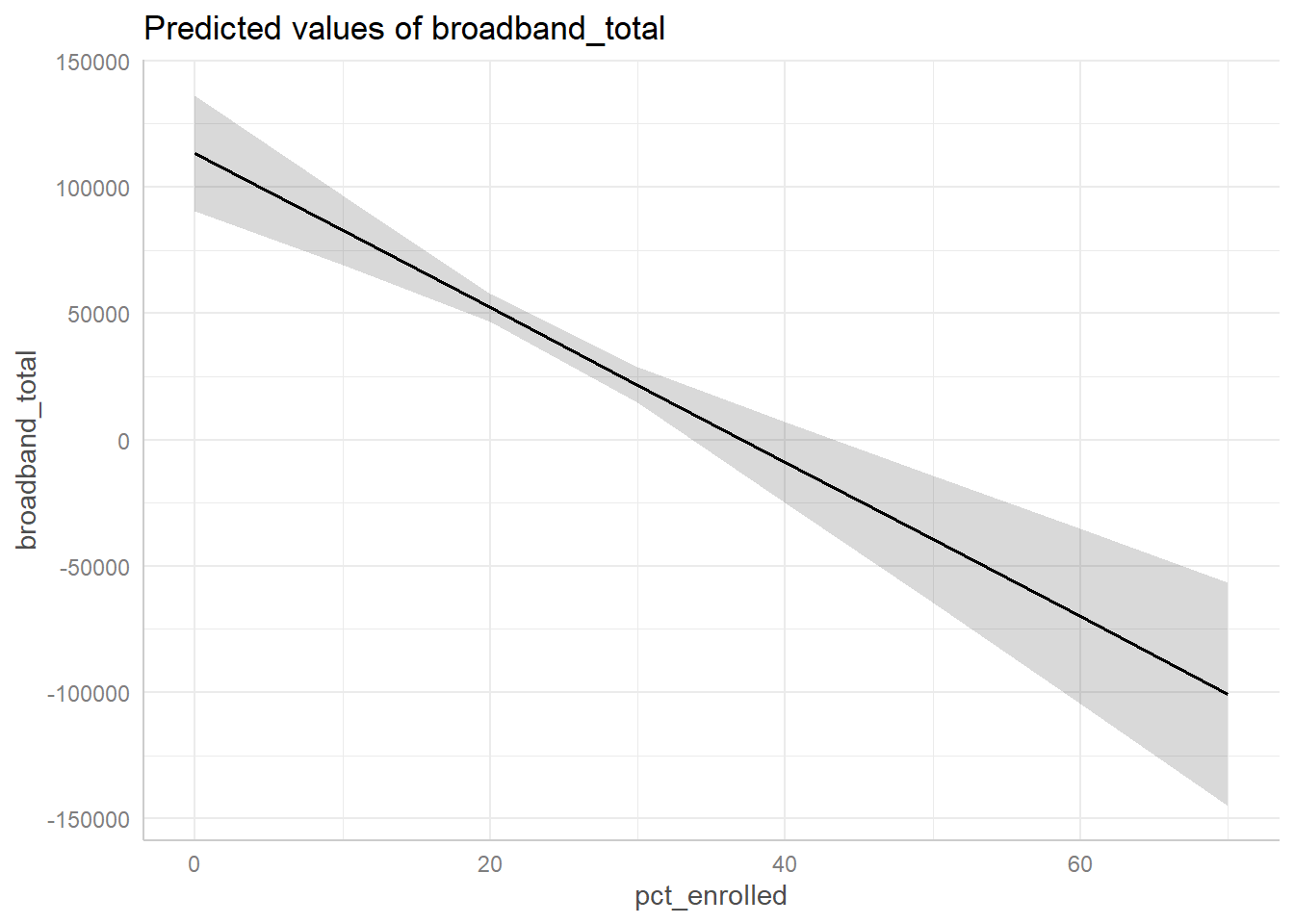
Percentage of individuals currently enrolled in school.
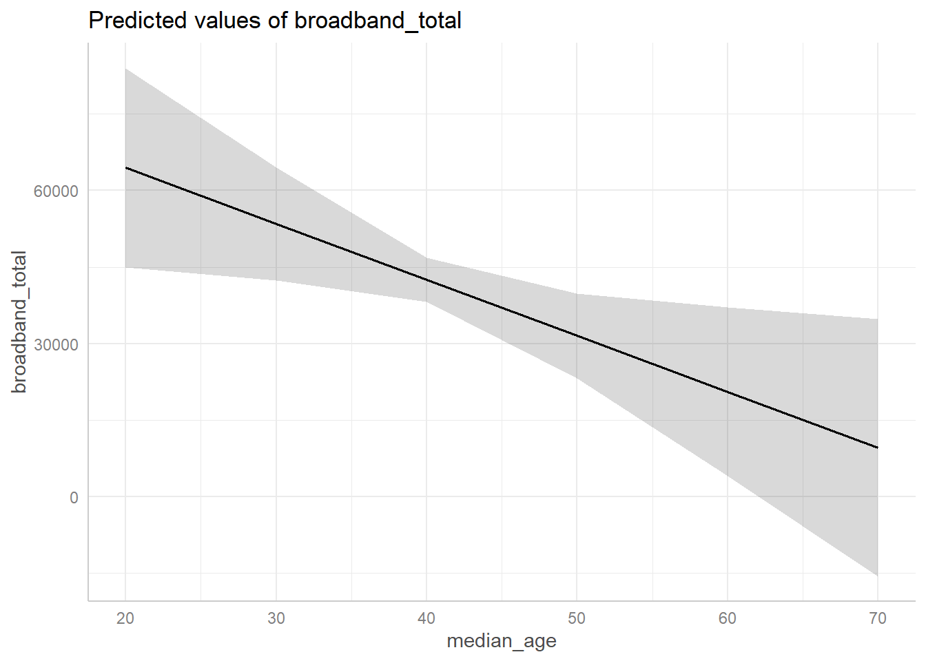
Median age of the population..

Model Formula

\[ \text{Broadband Access} = \beta_0 + \beta_1 \cdot \text{Income} + \beta_2 \cdot \text{White} + \beta_3 \cdot \text{Bachelor's Degree} + \beta_4 \cdot \text{School Enrollment} + \beta_5 \cdot \text{Age} + \epsilon \]

\[ \text{Broadband Access} = 209616.6 + 2343.0 \cdot \text{Income} + 415.3 \cdot \text{White} - 2345.0 \cdot \text{Bachelor's Degree} - 3056.9 \cdot \text{School Enrollment} - 1097.0 \cdot \text{Age} + \varepsilon \]

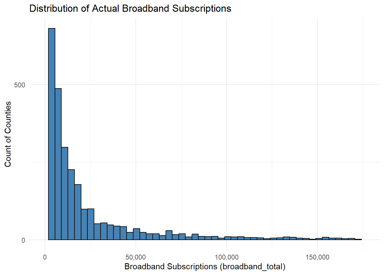
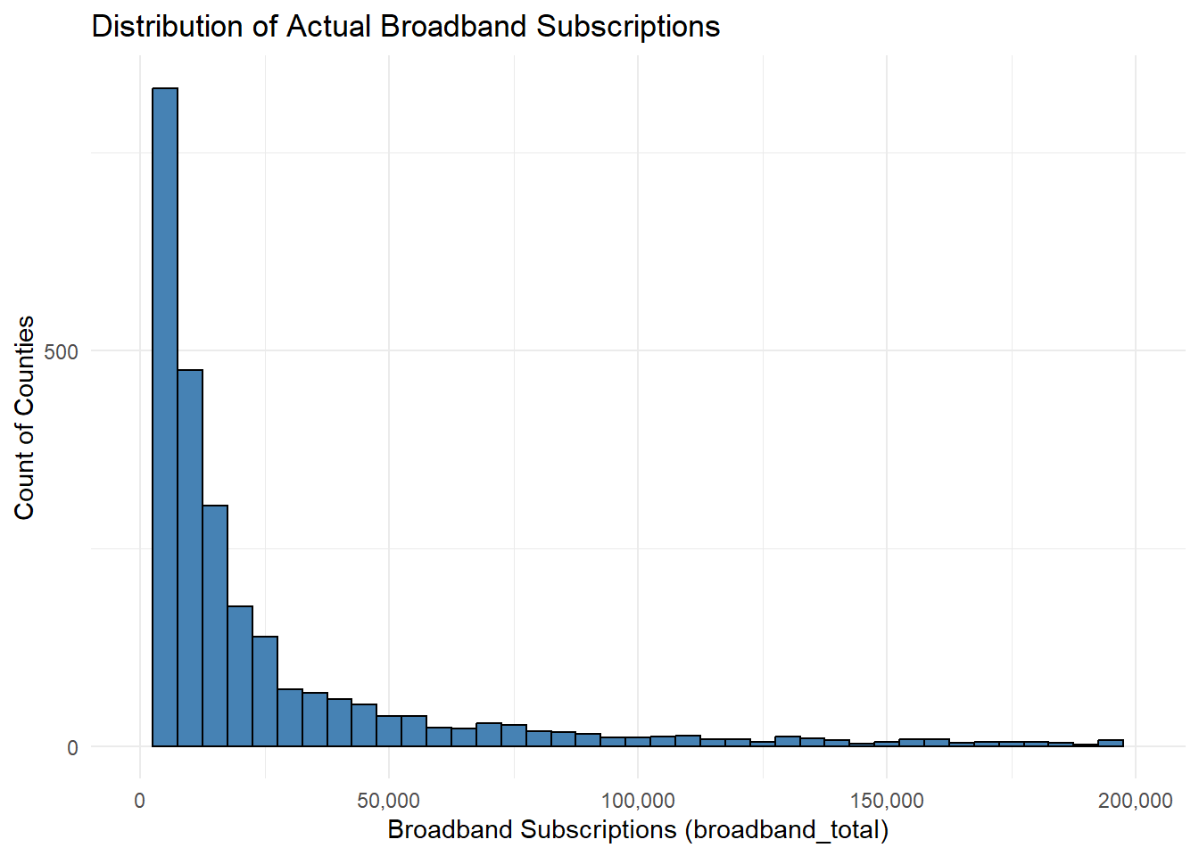
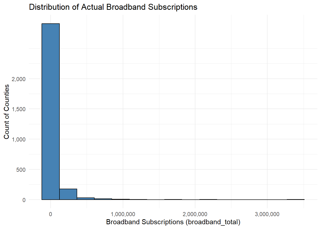
Data Preparation


Call:
lm(formula = broadband_total ~ median_income_k + pct_white + 
    pct_bachelor + pct_enrolled + median_age, data = acs_clean)

Residuals:
    Min      1Q  Median      3Q     Max 
-222384  -34847  -11657    9889 3255595 

Coefficients:
                Estimate Std. Error t value Pr(>|t|)    
(Intercept)     209616.6    44743.0   4.685 2.92e-06 ***
median_income_k   2343.0      145.2  16.137  < 2e-16 ***
pct_white          415.3      204.9   2.027   0.0428 *  
pct_bachelor     -2345.0      527.5  -4.446 9.07e-06 ***
pct_enrolled     -3056.9      485.3  -6.299 3.40e-10 ***
median_age       -1097.0      448.8  -2.445   0.0146 *  
---
Signif. codes:  0 '***' 0.001 '**' 0.01 '*' 0.05 '.' 0.1 ' ' 1

Residual standard error: 115400 on 3134 degrees of freedom
Multiple R-squared:  0.1214,    Adjusted R-squared:   0.12 
F-statistic: 86.63 on 5 and 3134 DF,  p-value: < 2.2e-16


Call:
lm(formula = broadband_total ~ median_income_k + pct_white + 
    pct_bachelor + pct_enrolled + median_age, data = acs_clean)

Residuals:
    Min      1Q  Median      3Q     Max 
-222384  -34847  -11657    9889 3255595 

Coefficients:
                Estimate Std. Error t value Pr(>|t|)    
(Intercept)     209616.6    44743.0   4.685 2.92e-06 ***
median_income_k   2343.0      145.2  16.137  < 2e-16 ***
pct_white          415.3      204.9   2.027   0.0428 *  
pct_bachelor     -2345.0      527.5  -4.446 9.07e-06 ***
pct_enrolled     -3056.9      485.3  -6.299 3.40e-10 ***
median_age       -1097.0      448.8  -2.445   0.0146 *  
---
Signif. codes:  0 '***' 0.001 '**' 0.01 '*' 0.05 '.' 0.1 ' ' 1

Residual standard error: 115400 on 3134 degrees of freedom
Multiple R-squared:  0.1214,    Adjusted R-squared:   0.12 
F-statistic: 86.63 on 5 and 3134 DF,  p-value: < 2.2e-16

# A tibble: 6 × 7
  term            estimate std.error statistic  p.value conf.low conf.high
  <chr>              <dbl>     <dbl>     <dbl>    <dbl>    <dbl>     <dbl>
1 (Intercept)      209617.    44743.      4.68 2.92e- 6 121888.    297345.
2 median_income_k    2343.      145.     16.1  2.46e-56   2058.      2628.
3 pct_white           415.      205.      2.03 4.28e- 2     13.5      817.
4 pct_bachelor      -2345.      527.     -4.45 9.07e- 6  -3379.     -1311.
5 pct_enrolled      -3057.      485.     -6.30 3.40e-10  -4008.     -2105.
6 median_age        -1097.      449.     -2.44 1.46e- 2  -1977.      -217.